How EV Dashboard measures efficiency and estimates range
A walkthrough of the math, written for owners and testers who want to know exactly what the numbers on screen are made of.
Version: 2026-08-25 · Applies to: app version 3.0 (build 146) and later
Overview
Your vehicle already shows a range distance and rolling efficiency on the instrument cluster, but I have found that very often these values do not match what I attained in real-world driving. I wanted to see if I could improve upon this, plus I wanted to enable some new features such as estimating your arrival state of charge (SoC) during a journey.
A caveat while it is fresh: the range estimates in my new 2026 IONIQ 5 seem better — my early impression is that they land closer to actual obtained range than I experienced with my 2024 IONIQ 5 — though I need to spend more time with the 2026 to form a more informed opinion.
Several new capabilities have been added to EV Dashboard. The app derives range and efficiency from signals it polls out of the battery management system (BMS) and the vehicle control unit (VCU), combined with GPS signals from your mobile device. Part 1 shows each of them on screen; Part 2 works through the math behind them.
This paper explains what the app’s numbers actually mean and how they are calculated, so you can judge which one is answering the question you are asking.
Part 1 — What the app shows you
The Range & Efficiency tile
Most of the app’s driving work ends up on one tile. It lives on the CarPlay dashboard, in whichever slot you have put it.
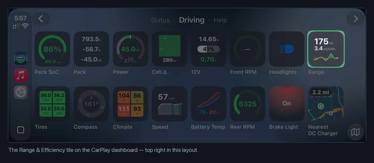
It is carrying three things at once: how far you can go, how efficiently you are going, and how that efficiency has been trending.
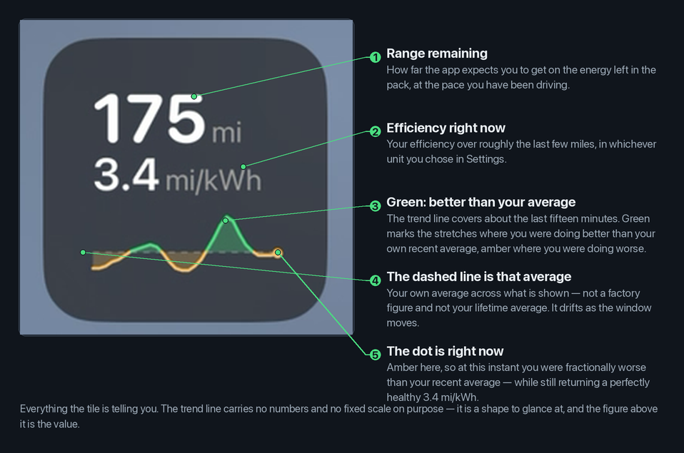
The trend line compares you against yourself
The green-and-amber trend line is the part most worth explaining.
The dashed line running across it is your own average over the fifteen minutes on display. It is not a factory figure, not a target, and not your lifetime average. Green marks the stretches where you were beating that average and amber the stretches where you were not — and that holds whichever efficiency unit you have chosen. If you display miles per kWh, better means higher, so green sits above the line; if you display Wh/km or kWh/100km, better means lower, and green sits below it. Green always means better than you had been doing, so you never have to remember which direction is good for your unit.
Two things are worth knowing before you read too much into the shape:
- There is no fixed scale, and no zero. The trend line stretches vertically to fit whatever is currently in it, so a very steady drive and a wildly varying one can look about equally dramatic. Read the trend line for the pattern — am I trending better or worse, and where did that turn? — and read the number above it for the value.
- The average you are measured against moves. Because the dashed line is the average of the very stretch being coloured, there is always some green and some amber. You cannot drive your way to an all-green trend line, and a long, efficient descent will drag the average down far enough to turn ordinary cruising amber.
What reliably moves it: hills, speed, outside temperature, cabin heating or cooling, and stop-and-go traffic. A long descent on regenerative braking can push it deep into green.
If the trend line is blank, it simply has not collected enough yet. It needs a couple of minutes of driving, fills in from the left, and a short stop does not wipe it.
Estimated arrival state of charge
Set a destination and the app will tell you what it expects to be left in the pack when you get there.
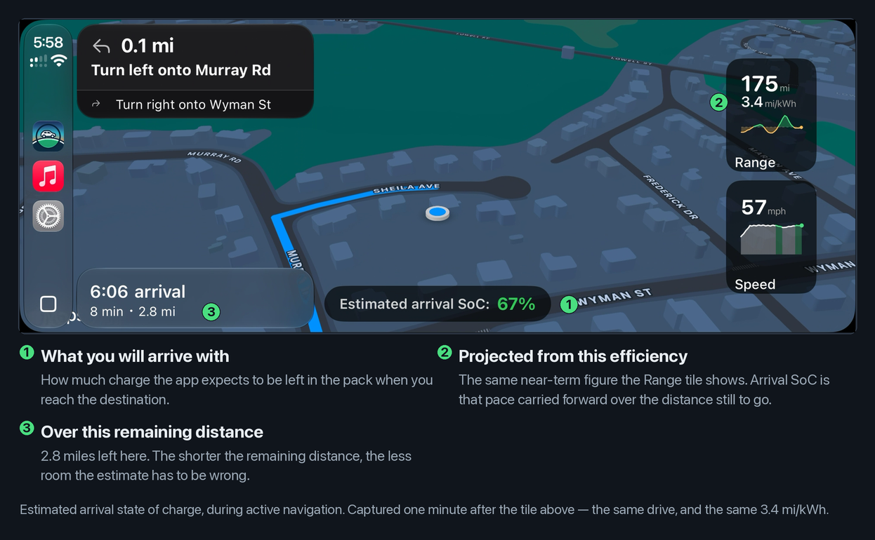
The arithmetic is deliberately plain: the app takes the pace you have actually been driving, carries it forward over the distance still to go, and subtracts the result from what is in the pack now. There is no route lookahead behind it — no elevation model, no speed limits, no weather.
That has a practical consequence worth internalising. The estimate is at its weakest at the very start of a journey whose character is about to change — a mountain pass immediately after city driving is the classic case — and it corrects itself as you go, because the pace it is extrapolating from catches up with the new road while the distance it is extrapolating over shrinks. A number that looks alarming in the first mile is usually worth re-reading five miles later.
Your efficiency for a drive
When a drive ends, the app records it. Opening it in History gives you the whole-drive figure.
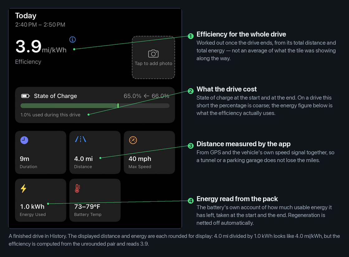
This is a different number from the one the tile was showing while you drove, and the difference is the point. The tile answers how am I driving right now, over roughly the last few miles. The session answers how efficient was that drive, over all of it. A drive that started cold and finished on a warm highway will show a session figure somewhere between the two extremes the tile passed through.
One detail that trips people up: the three numbers here are rounded independently for display, and the efficiency is worked out before any of that happens. Above, 4.0 mi divided by 1.0 kWh looks like it should read 4.0 — but the drive used a little over 1 kWh, which displays as “1.0”, while the efficiency is calculated from the full figure. Rounding once at the end is deliberate: working from the already-rounded numbers would make the efficiency itself less accurate. The gap only shows on very short drives, where a hundredth of a kWh is a large share of the total.
Which number answers which question
There are three efficiency figures which represent different things.
| Number | Where you see it | What it answers |
|---|---|---|
| Trip efficiency | History ▸ a driving session | “How efficient was that drive?” |
| Near-term efficiency | The Range tile and its trend line | “How efficient am I driving right now?” |
| Long-term efficiency | Nowhere — it divides into Range and arrival SoC | “What should I expect over the miles ahead?” |
The third one never appears on screen anywhere, and it is the one that moves your range. Part 2 explains why the app keeps two horizons of the same measurement rather than one.
Part 2 — How the numbers are calculated
1. Notation and units
The app works internally in metric canonical units and converts only at display time.
| Symbol | Meaning | Canonical unit |
|---|---|---|
| Energy | kilowatt-hours (kWh) | |
| Distance | kilometres (km) | |
| Pack power | kilowatts (kW) | |
| Near-term efficiency (consumption form) | watt-hours per kilometre (Wh/km) | |
| Long-term efficiency — the range divisor (§4.4) | watt-hours per kilometre (Wh/km) | |
| State of charge | percent (%) | |
| Available pack energy | kWh |
The single conversion constant used throughout:
Display units
You choose the efficiency unit in Settings ▸ Units ▸ Efficiency. It is independent of your distance unit, so a metric driver can read distance in km and consumption in kWh/100km. All five forms are conversions of the same underlying Wh/km value:
| Selected unit | Formula from the canonical pair | From in Wh/km | Direction |
|---|---|---|---|
| mi/kWh | higher is better | ||
| km/kWh | higher is better | ||
| kWh/100km | lower is better | ||
| Wh/mi | lower is better | ||
| Wh/km | lower is better |
Worked conversion. An efficiency of Wh/km displays as:
The two “rate” forms (distance per energy) improve as they rise; the three “consumption” forms (energy per distance) improve as they fall. The app tracks that polarity so the CarPlay trend line tints green for “better than your recent average” in whichever unit you picked.
Rounding: Wh/mi and Wh/km display as whole numbers; the other three display to one decimal.
2. Three efficiency values, one of them invisible
Part 1 set out the three figures and where each one appears. Two of them you can see; the third never appears on screen, but it is the one that moves your range.
All three are consumption figures (energy per distance), and all three read energy from the same place — the battery’s own account of how much usable energy it has left. They differ only in the span they cover: one whole drive, the last few miles, or a horizon several times longer than that. Near-term and long-term are computed from exactly the same measurements and differ by a single constant; §4.4 explains why the app keeps both.
3. Trip efficiency
This is the headline number on every completed driving session. It is derived at display time from two values stored as part of the session record:
where is whichever display formula from §1 you selected.
3.1 The energy term — read from the pack, not calculated
The app reads the BMS’s own available-energy report at the start and end of the drive and takes the difference:
is availableEnergy, decoded from BMS diagnostic identifier 0x0105 which is polled every 30 seconds.
Two raw bytes at offset 28, scaled:
Three properties follow from using the BMS accounting:
- Regeneration is netted automatically. Energy recovered on a downhill run raises available energy, which shrinks the difference.
- Everything on the high-voltage bus is included — traction motor drive, climate control, battery conditioning, the DC-DC converter feeding the 12 V system.
- Pack capacity, degradation, and temperature are already baked in, because the BMS computes available energy against the real pack.
3.2 The distance term
Trip distance is measured as a speed integral over the session timeline:
That is a trapezoid rule: each new speed sample credits the time since the last one, at the average of the two speeds.
Two independent speed channels feed it:
- Doppler speed from GPS fixes on your mobile device (~1 Hz). A fix credits distance only if it passes a confidence gate: reported speed and its stated speed accuracy is m/s. This is the fix’s own reported speed, never derived by differencing positions — so it does not jitter while parked and has no scale bias.
- Vehicle speed from the VCU, polled roughly every 2.5–3 seconds. It credits only the intervals Doppler has not already covered — specifically, when no confident fix has arrived within the last 2.5 seconds. This carries the drive through tunnels, parking garages, dead GPS, or denied location permission.
Every second of the session is attributed to exactly one of four buckets — doppler, wheel, stationary, or gap — and nothing is silently dropped.
A single timeline marker guarantees no interval is ever counted twice.
Interval rules:
| Rule | Value | Effect |
|---|---|---|
| Credit cap | 10 s | A sample arriving 14 s after the marker credits 10 s and books 4 s as gap — no data means no invented distance |
| Stationary floor | 0.15 m/s | Below this the interval is verified stationary: time counted, zero distance. A stopped car is a measurement, not a gap |
| Doppler freshness | 2.5 s | How long a confident fix suppresses the vehicle-speed channel |
| Doppler confidence gate | 2.0 m/s | Fixes with worse stated speed accuracy do not credit |
Worked micro-example. Cursor anchored at with ; times in seconds, speeds in m/s:
3.3 Coverage, and when the odometer gets a vote
At session close the app computes how much of the drive it actually measured:
Then a single decision:
Worked example. A 37-minute drive attributes 1,510 s to Doppler, 240 s to vehicle speed, 380 s stationary, 95 s gap:
Why the odometer is inadequate as the primary source. The car’s odometer signal reports in whole miles or whole kilometers. A real-world short 1.443 km errand quantizes to 1.609 km — an 11 % error on that trip, and much worse on shorter ones. Measured on one verification drive (2026-07-21), the integral gave 1.443 km against a 1.609 km odometer delta, with 98 % coverage. The odometer is therefore a coverage-gated fallback, never an arbiter of a well-measured drive.
3.4 Putting it all together
Sample trip. Available energy 61.4 kWh when the car was put into gear, 53.3 kWh at ignition-off; the integral measured 42.0 km at 96 % coverage.
During the drive the app shows the running integral live; the coverage gate is applied once, when the session ends.
4. Rolling efficiency
Rolling efficiency is a rate that reflects how you are driving now rather than how you drove an hour ago. This is a separate estimator with its own energy and distance measurements.
Everything in §4.1 to §4.3 describes a single measurement pipeline: one window, one sample, one plausibility band. Section 4.4 is where that single stream becomes the two figures of §2 — near-term and long-term — which differ only in how quickly each forgets.
4.1 Energy
Similar to trip efficiency, energy comes from the battery’s own available-energy reading, differenced between the start and end of a measuring window:
The reading resolves to 0.002 kWh (2 Wh) and is polled every 30 seconds, so a minute of driving typically moves it by several dozen steps — fine enough to measure against, provided the window is long enough. §4.3 explains why that qualifier matters.
Idling still costs you, exactly as you would expect: sitting at a red light with the climate control running keeps draining the pack, so available energy keeps falling while the distance term does not grow. The window that eventually closes has that consumption in it.
4.2 Distance
Distance is measured the same as trip efficiency — the same running total, from the same two speed sources, produced by the same code. The rolling estimate simply reads how far that total has advanced since its own measuring window opened.
Why a window can be thrown away. There is one thing the rolling figure must do that the trip total does not, and it follows from the energy side rather than the distance side. The distance totalizer tracks how much of the drive it could not account for. When that unaccounted time grows during an open rolling efficiency time window, the app abandons that time window and starts a fresh one rather than including a distorted measurement. The two cases where a window is abandoned. Note that a window is always discarded whole — its distance and its energy together — so the two halves always describe the same span of driving. Individual distance readings are never selectively dropped.
| Case | Trigger | Why |
|---|---|---|
| Unmeasured driving | More than 5 s of the time window went unaccounted for | Energy is complete but distance is short, so the window would read falsely inefficient |
| A new drive begins | The app is told a driving session has started | The open window described a different drive |
The second case is also what handles charging. Plugging in ends the driving session, so the reading taken before you charged is discarded when you next set off — the app does not watch for the charger separately.
A stop does not abandon a window, deliberately. Sitting in traffic or idling with the climate running spends real energy over no distance, and that is exactly what your efficiency should reflect. The energy keeps accruing against the open window and lands in the next measurement, so a long wait shows up as worse efficiency. A rise in available energy while you are moving is regeneration — real driving data, and kept.
When a window is abandoned. A window is only abandoned when both the phone’s GPS and the car’s speed signal go quiet at once.
4.3 The blend — a distance-weighted exponential moving average
The estimator keeps one measuring window open at a time, accumulating distance (km) and energy (kWh). When the window is big enough it closes, produces one sample, and a fresh window opens:
is the fraction of the old estimate retained. The exponent’s denominator is the half-life: 8 km (about 5 miles).
Update cadence: All three of these must be true, so the estimate updates at most once a minute:
| Condition | Value | What it prevents |
|---|---|---|
| Time since the window opened | ≥ 60 s | Updating so often that noise dominates the measurement |
| Distance measured | ≥ 0.3 km | Dividing a real energy reading by a few metres of GPS wobble |
| Energy moved | ≥ 0.05 kWh | Folding a zero while the battery’s reading sits between updates |
The three conditions also mean the display simply holds its last value in stop-and-go traffic rather than reporting noise: if the car has not covered 300 meters, the window stays open until it does.
Example calculation: Begin with a starting estimate of 200 Wh/km followed by the car covering 2.0 km with the the battery’s available energy falling by 0.5 kWh:
How the exponential moving average works. The obvious way to average recent driving would be to take the last few miles and average them evenly — but that has an awkward edge. A measurement counts fully right up until it falls out of the window, then counts for nothing at all. Drive past that boundary and the display lurches, for no reason connected to how you are driving.
An exponential moving average has no window and no boundary. Instead of storing past measurements, it keeps a single running number and nudges it toward each new measurement:
If were 0.9, each new measurement would move the estimate a tenth of the way toward itself and leave nine tenths of what was already there. Nothing is ever dropped; older driving simply fades, its influence shrinking a little with every update. That is what makes the display move smoothly instead of stepping.
Why the nudge size depends on distance. A measurement covering 2 km deserves more say than one covering 300 m, so is not a fixed number — it is computed from the distance that window covered:
Read it as: every 8 km of driving cuts the influence of everything that came before it in half. That is what “half-life” means here. Drive 8 km and the past counts half as much; drive another 8 and it counts a quarter as much. It never reaches zero — it just becomes too small to matter.
| Distance since a measurement | Weight it still carries |
|---|---|
| 8 km (5 mi) | 50 % |
| 16 km (10 mi) | 25 % |
| 24 km (15 mi) | 12.5 % |
| 40 km (25 mi) | 3 % |
What that looks like on the display. Suppose you have been driving in town at 150 Wh/km and you join the highway, where you settle at 200 Wh/km. The figure does not jump to 200, and it does not wait and then snap — it slides:
| After this much highway | Displayed |
|---|---|
| 0 km | 150 Wh/km |
| 4 km (2.5 mi) | 165 Wh/km |
| 8 km (5 mi) | 175 Wh/km |
| 16 km (10 mi) | 188 Wh/km |
| 24 km (15 mi) | 194 Wh/km |
| 40 km (25 mi) | 198 Wh/km |
Most of the change lands in the first ten miles, and the last few percent take a while — which is the intended behavior. The number is meant to answer “how am I driving lately”, so it should move decisively when your driving genuinely changes and ignore the fact that you just went up one hill.
Why 8 km. It is long enough that a single hill, one traffic light, or a brief burst of acceleration cannot move the figure much, and short enough that a real change of road or driving style shows up within a few miles rather than at the end of the trip.
Why weight by distance rather than time. A 20-minute crawl through traffic and 20 minutes of highway cruising are not equally informative about the next 100 miles. Distance weighting means a slow crawl cannot dominate the average, and a fast highway stretch is not underweighted just because it took less time.
The plausibility band (−200 to 5000 Wh/km) rejects readings that cannot be real. The two ends guard different things, which is why they are not symmetric. The low end is a physical limit on how much energy regeneration can return over a kilometer; anything beyond it is a data fault rather than a descent. The high end has to be generous, because a genuinely large reading is easy to produce honestly: sit at a level crossing for twenty minutes with the climate running, then move off, and the first 300 meter carry twenty minutes’ worth of energy.
The 40 Wh/km limit guards something different from the band above: the band bounds a single measurement, this bounds the running average itself. Range is available energy divided by efficiency, so a long descent that dragged the average to zero would leave the division with no answer at all, and below zero it would produce a negative range. The limit prevents that.
Whether it reads as a floor or a ceiling depends on your chosen unit — 40 Wh/km is the same limit as 15.5 mi/kWh — but on range it is always a ceiling: at that efficiency a 60 kWh pack would project around 1,500 km.
That figure is the point. This is a mathematical guard, not a plausibility one: 40 Wh/km is about four times better than any production EV achieves, so if the average ever reaches the limit the range shown will be wildly optimistic — finite, but not to be relied on. It recovers within a few miles of the road flattening out.
4.4 Two horizons from one measurement
Everything above produces one sample per closed window. That sample is folded twice, into two running averages that differ only in half-life:
| Half-life | Where it goes | |
|---|---|---|
| Near-term | 8 km | The efficiency number on the Range tile, and the trend line beneath it |
| Long-term | 60 km | The range figure (§5) and arrival state of charge (§6) |
There is no second measurement and no second window — the same energy, the same distance, the same plausibility band and limit. Only the blending constant differs.
Why two. An efficiency readout and a range estimate are answering different questions, and the honest answer to each has a different shape. “How am I driving?” is about the last few miles, and should move when the road changes. “How far can I get?” is about the miles ahead, and a figure that lurches every time you crest a hill is not describing them.
A round trip on 1 August 2026 made the cost of conflating them concrete. The two legs covered the same road within a few hours of each other, and their true whole-drive efficiencies were 169 and 168 Wh/km — the same drive, twice. The 8 km average finished those legs reading 147 and 202 Wh/km, because one ended on a highway descent and the other on town streets. Neither reading was wrong about the miles it described. Both were poor divisors for the pack.
Dividing by them produced a range figure that rose by a total of 462 km on the outbound leg and 346 km on the return, in individual jumps as large as 85 km — while the car was being driven steadily in one direction. On the same drives, the 60 km average holds those totals to 49 km and 40 km, with worst jumps of 4 km and 11 km.
What it costs. A genuine, sustained change of conditions — a mountain pass, a headwind, winter — takes about 60 km to half-register in the range figure. That is the deliberate trade: the near-term number still shows such a change within a few miles, so the information is on screen immediately, just not in the division.
A consequence worth expecting. The efficiency number and the range can now move independently, and sometimes visibly disagree — efficiency dropping while range holds steady. That is the design working, not a fault.
4.5 Where the estimate starts
The estimator is seeded from your own last drive, stored per vehicle (keyed by VIN) and saved every 10 seconds while driving:
The stored seed is applied when nothing has been measured this drive (less than 0.2 km), so a VIN that resolves mid-drive cannot overwrite live measurement with yesterday’s number. The fixed 207 Wh/km baseline is only used as the first-ever-drive starting point.
4.6 One measurement, two spans
Both efficiency figures are built from the same two ingredients: the battery’s available-energy reading and the distance engine. The only thing that differs is the span each one covers.
| Trip efficiency | Near-term efficiency | |
|---|---|---|
| Energy | Available-energy delta | Available-energy delta |
| Distance | The totalizer of §3.2 | The totalizer of §3.2 |
| Span | The whole drive, start to finish | A rolling weighted average of roughly the last 5 miles |
| Long-term twin | — | The same stream at a 60 km half-life (§4.4) |
| Incomplete stretches | Accounted for and reported as coverage; the odometer can stand in | The affected window is abandoned |
That means the two numbers cannot disagree about what was measured — only about how much of the drive they are describing. Finish a drive that started in city traffic and ended on the highway, and the trip figure will report the average of the whole thing while the near-term figure ends up near the highway portion. Both are right; they are answering different questions.
5. Range
5.1 The formula
where is the BMS’s reported available pack energy in kWh and is the long-term efficiency in Wh/km — the 60 km average of §4.4, not the number shown beside the range. In miles, multiply by 0.621371 — which the app does at display time, rounding to a whole unit.
Worked example. Available energy 52.0 kWh, long-term efficiency 185 Wh/km:
5.2 When the number updates
Range has two independent inputs, and each refreshes it on its own schedule:
- Long-term efficiency changes only while the vehicle is moving, and at most once a minute (§4.3). Each update moves it slightly, because a single window is a small fraction of a 60 km half-life (§4.4).
- Available energy changes on every BMS poll — roughly every 30 seconds — including while parked and while charging.
Between the two, available energy is now the faster-moving term, which is why the range figure reads as a countdown: most of what you see is the pack draining, not the model changing its mind.
So the range figure is live from the first BMS poll after the app connects, without needing any location data, and it climbs while you charge. If the BMS has not reported energy yet (or reports 0.1 kWh or less), range renders as a dash rather than a guess.
6. Arrival state of charge
When a route is active, the app shows the one number the car’s own navigation cannot: the state of charge you should arrive with.
The derivation is simple proportionality: is the fraction of your remaining usable energy the trip will consume, so is the fraction left, and scaling today’s SoC by it gives the arrival SoC.
Arrival SoC uses for the same reason range does: it is a projection across every remaining mile of the route, so it takes the long-horizon figure rather than the one describing the last few (§4.4).
Worked example. SoC 68 %, available energy 52.0 kWh, 120 km remaining, efficiency 185 Wh/km:
is the distance to the current turn plus the sum of all later steps, recomputed on every GPS fix by the app’s own trip engine — so it keeps counting even when CarPlay’s guidance panels are suspended.
The projection is worked out once a minute, and what you see is an average of the last five.
It is unusually sensitive to the efficiency figure: once a leg needs most of the pack, a 10 % change in efficiency moves the arrival estimate by around 5 percentage points. Shown unsmoothed, that arrives as a single jump. Averaging the last five minutes turns the same 5-point move into five 1-point steps.
The averaging costs less than it might appear, because this figure does not drift as you drive. Drive at exactly the efficiency it assumes and it holds the same value the entire way: your state of charge falls, the energy left falls, and the distance still to go falls, and those changes cancel out.
| After driving | Remaining | SoC now | Arrival SoC |
|---|---|---|---|
| 0 km | 120 km | 68 % | 39 % |
| 40 km | 80 km | 58 % | 39 % |
| 80 km | 40 km | 49 % | 39 % |
| 120 km | 0 km | 39 % | 39 % |
So the estimate only moves when your actual driving differs from what was predicted — which is exactly the change worth smoothing rather than reacting to instantly. The real cost is response time: if conditions genuinely change, the arrival figure takes the full five minutes to catch up.
A new destination or a reroute starts a fresh average rather than blending two journeys.
The displayed value is tinted green at 20 % or above, amber from 10 % to 20 %, and red below 10 %.
7. What the model does not do
These are some things the model does not factor in, but may be explored in the future.
- No route lookahead. The estimate extrapolates “how you have been driving” over “the distance that remains”. There is no elevation model, no speed-limit model, no weather model. It is least accurate at the start of a trip whose character differs sharply from the last few miles, e.g., a mountain pass right after city driving — and it self-corrects as the moving average absorbs the new pace and the remaining distance shrinks.
- No odometer in the rolling estimate. Whole-mile/kilometer quantization is uselessly coarse against an 8 km averaging window: an entire half-life fits inside one odometer tick.
- No reading of the car’s own range estimate. This is not a known signal over the OBD-II port.
8. Constants reference
Every tunable that affects a number in this paper.
Rolling efficiency estimator (near- and long-term)
| Constant | Value | Meaning |
|---|---|---|
| Cold-start baseline | 207 Wh/km | First-ever-drive seed (≈ 3.0 mi/kWh) |
| Seed plausibility band | 60–600 Wh/km | A stored value outside this is discarded |
| Seed cutoff | 0.2 km | Past this measured distance, a late seed is not applied |
| Persist cadence | 10 s | How often the estimate is saved while driving |
| Near-term half-life | 8.0 km | The newest ~5 miles carry half the displayed figure |
| Long-term half-life | 60 km | The range and arrival-SoC divisor (§4.4) |
| Confidence threshold | 1.6 km | Internal flag only; not surfaced |
| Unmeasured time allowed | 5 s | More than this inside a window abandons it |
| Minimum window time | 60 s | The estimate updates no more often than this |
| Minimum window distance | 0.3 km | Below this the window stays open |
| Minimum window energy | 0.05 kWh | Below this the window stays open |
| Plausibility band | −200 to 5000 Wh/km | Readings outside this cannot be real |
| Efficiency limit | 40 Wh/km | Bounds the running average so the range division always has an answer |
Trip distance engine
| Constant | Value | Meaning |
|---|---|---|
| Doppler confidence gate | 2.0 m/s | Max stated speed uncertainty that still credits |
| Doppler freshness | 2.5 s | How long a good fix suppresses the vehicle-speed channel |
| Credit cap | 10 s | Max time one sample can retroactively claim |
| Stationary floor | 0.15 m/s | Below this: covered time, zero distance |
| Coverage floor | 0.80 | Below this, fall back to the odometer delta |
Signals
| Signal | Source | Cadence | Resolution |
|---|---|---|---|
| Available energy | BMS diagnostic ID 0x0105 | 30s | 0.002 kWh |
| State of charge | BMS diagnostic ID 0x0105 | 30s | 0.5 % |
| Vehicle speed | VCU | ~2.5–3s | 1/64 km/h |
| GPS fixes | Mobile device | ~1 Hz while a drive session is active | — |
9. Reading the drive recorder log
Everything described in this paper writes to one file, and you do not have to remember to start it. The Drive Diagnostics Recorder (Settings ▸ Diagnostics) is on by default and writes a separate flight-recorder file for each drive; the newest ten are kept, and Share Drive Diagnostics hands you the most recent one.
The line format
Every line is one event:
t=+842.113 [ENERGY] evt=energy eff=185 range=281 conf=1 distKm=42.30 …
tis seconds since the recording started — the absolute start time is in the file header, so every line in the file shares one clock[TAG]names the subsystem, the same bracketed convention the app’s other logs useevtnames the record type, and everything after it iskey=value
Values never contain spaces, so the whole file can be read with a text editor’s search, or split on spaces by any script.
Four tags appear:
| Tag | Covers |
|---|---|
[GPSDIST] |
The distance engine — GPS fixes, wheel-speed samples, odometer readings, and the close decision |
[ENERGY] |
Near- and long-term efficiency, range, and arrival state of charge |
[NAV] |
Turn-by-turn guidance — routing, maneuvers, reroutes |
[TRACE] |
The recording itself — start, end |
The point of one file rather than several is that these share a timeline. When an efficiency window is discarded you can read straight across to the fixes that caused it, instead of correlating two logs by wall-clock time.
The efficiency record
[ENERGY] evt=energy — one state line every 30 seconds while moving, every 5 minutes while stopped:
t=+842.113 [ENERGY] evt=energy eff=185 rangeEff=178 range=292 conf=1 distKm=42.30
pendKm=0.180 pendKWh=0.031 soc=68.0 availE=52.014 folds=37 reanch=4 clamps=0 gaps=2
eff— near-term efficiency in Wh/km: the number on the Range tilerangeEff— long-term efficiency (§4.4), the valuerangewas actually divided by. The gap betweeneffandrangeEffis the smoothing; on a steady drive they converge, and on a changing one they should differrange— in km, before any unit conversion for displayconf— whether the 1.6 km confidence threshold has been passed (the internal flag in §8)distKm— measured distance this drive, taken from the shared totalizer that also builds the trip figure (§4.2)pendKm/pendKWh— the window currently open: how much distance and energy have accrued toward the next updatefolds— how many windows have closed and entered the moving averagereanch— windows excluded by the distance engine (gap, or before drive start) A high count relative tofoldsmeans the drive was measured in fragments — worth knowing before trusting the figureclamps— readings that fell outside the plausibility bandgaps— unmeasured stretches that forced a re-anchor
availE is logged to three decimals because that is the signal’s real resolution.
Four one-off [ENERGY] records fill in the rest: energy_params stamps every constant in §8 at the start of the drive, so an old file stays interpretable after the constants are retuned; energy_reanchor, energy_clamp, and energy_confident each record the moment they happen, with the values that caused them.
The distance record
[GPSDIST] evt=close — one line per drive, recording the distance decision:
t=+2431.007 [GPSDIST] evt=close endReason=ignition_off integKm=42.031 cov=0.960
odoDeltaKm=41.843 chose=INTEGRAL distanceKm=42.031 startSoC=84.0 endSoC=68.0 energyKWh=7.79
The choice between the integral and the odometer is always recorded (§3.3), alongside the start and end values the trip figures are built from.
Before it, evt=fix carries every GPS fix with its stated confidence and crediting verdict, evt=wheel every vehicle-speed sample, and evt=buckets the final four-way attribution of §3.2 — so the coverage figure in the close line can be checked against the seconds that produced it.